Python中qutip用法示例詳解
前言
QuTip是用于模擬開放量子系統動力學的開源庫。QuTip庫依賴于的Numpy、Scipy和Cython的數值包。此外,matplotlib提供了圖形輸出。http://qutip.org/。
python安裝比較容易,需要選擇一個版本,python2或python3,稍微麻煩的是Scipy。
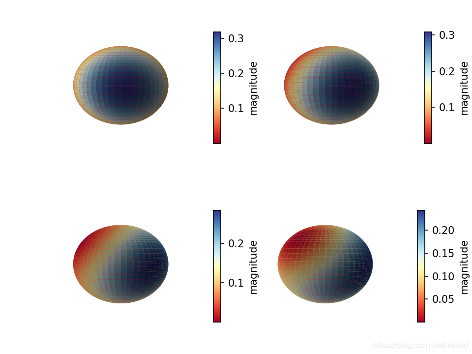
一、N原子系綜自旋概率分布
from qutip import *import numpy as npimport matplotlib.pyplot as pltn=2#原子數j = n//2psi0 = spin_coherent(j, np.pi/3, 0)#設置系統的初態為自旋相干態Jp=destroy(2*j+1).dag()#升算符J_=destroy(2*j+1)#降算符Jz=(Jp*J_-J_*Jp)/2#JzH=Jz**2#系統的哈密頓量tlist=np.linspace(0,3,100)#時間列表result=mesolve(H,psi0,tlist)#態隨時間的演化theta=np.linspace(0, np.pi, 50)phi=np.linspace(0, 2*np.pi, 50)#分別計算四個狀態下的 husimi q函數Q1, THETA1, PHI1 = spin_q_function(result.states[0], theta, phi)Q2, THETA2, PHI2 = spin_q_function(result.states[30], theta, phi)Q3, THETA3, PHI3 = spin_q_function(result.states[60], theta, phi)Q4, THETA4, PHI4 = spin_q_function(result.states[90], theta, phi)#在四個子圖中分別畫出四個狀態下的husimi q函數fig = plt.figure(dpi=150,constrained_layout=1)ax1 = fig.add_subplot(221,projection=’3d’)ax2 = fig.add_subplot(222,projection=’3d’)ax3 = fig.add_subplot(223,projection=’3d’)ax4 = fig.add_subplot(224,projection=’3d’)plot_spin_distribution_3d(Q1, THETA1, PHI1,fig=fig,ax=ax1)plot_spin_distribution_3d(Q2, THETA2, PHI2,fig=fig,ax=ax2)plot_spin_distribution_3d(Q3, THETA3, PHI3,fig=fig,ax=ax3)plot_spin_distribution_3d(Q4, THETA4, PHI4,fig=fig,ax=ax4)for ax in [ax1,ax2,ax3,ax4]: ax.view_init(0.5*np.pi, 0) ax.axis(’off’)#不顯示坐標軸fig.show()
運行結果:
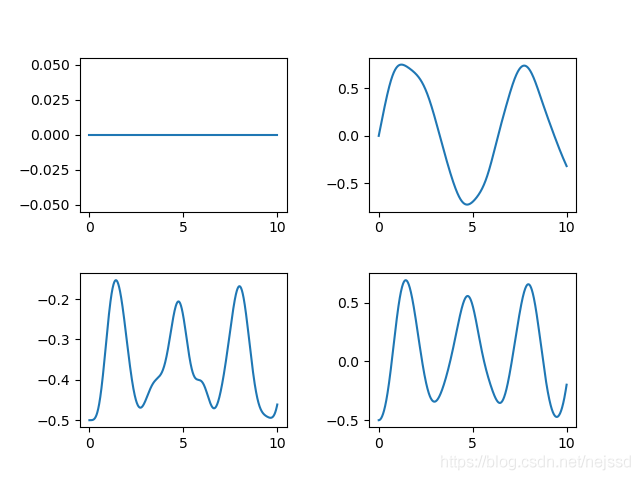
二、原子與光場相互作用
from qutip import *import numpy as npimport matplotlib.pyplot as pltalpha=1#相干光的參數alphan=2#原子數j = n/2psi0 = tensor(coherent(10,alpha),spin_coherent(j, 0, 0))#設置系統的初態a=destroy(10)#光場的湮滅算符a_plus=a.dag()#光場的產生算符Jp=destroy(n+1).dag()#原子的升算符J_=destroy(n+1)#原子的降算符Jx=(Jp+J_)/2#原子的Jx算符Jy=(Jp-J_)/(2j)#原子的Jy算符,這里的j是虛數單位Jz=(Jp*J_-J_*Jp)/2#原子的Jz算符H=tensor(a,Jp)+tensor(a_plus,J_)#系統的哈密頓量tlist=np.linspace(0,10,1000)#時間列表result=mesolve(H,psi0,tlist)#態隨時間的演化fig=plt.figure()ax1 = fig.add_subplot(221)ax2 = fig.add_subplot(222)ax3 = fig.add_subplot(223)ax4 = fig.add_subplot(224)ax1.plot(tlist,expect(tensor(qeye(10),Jx),result.states))#Jx的平均值隨時間變化圖ax2.plot(tlist,expect(tensor(qeye(10),Jy),result.states))#Jy的平均值隨時間變化圖ax3.plot(tlist,expect(tensor(qeye(10),Jz),result.states))#Jz的平均值隨時間變化圖ax4.plot(tlist,expect(tensor(qeye(10),Jx**2+Jy**2+Jz*2),result.states))#J平方的平均值隨時間變化圖fig.subplots_adjust(top=None,bottom=None,left=None,right=None,wspace=0.4,hspace=0.4)#設置子圖間距fig.show()
運行結果:
總結
到此這篇關于Python中qutip用法的文章就介紹到這了,更多相關Python qutip用法內容請搜索好吧啦網以前的文章或繼續瀏覽下面的相關文章希望大家以后多多支持好吧啦網!
相關文章:

 網公網安備
網公網安備